
We all recently heard that ChatGPT and GPT-3 were made based on an approach called Mixture of Experts (MoE). Such an approach has gained traction is the machine learning field which is a powerful paradigm that excels in handling complex, high-dimensional data. In this blog post, we embark on an enlightening step-by-step tutorial to develop, train, test, and validate a Mixture of Experts for the classification of images from the CIFAR-10 dataset.
To implement MoE for image classification, we leverage the CIFAR-10 dataset, a benchmark in computer vision. With 60,000 32x32 color images across 10 classes, CIFAR-10 is a challenging playground to showcase the capabilities of MoE.
By the end of this story, you will understand the basics of a Mixture of Experts, and how to develop a MoE for basic and simple classification problems.
P.S. This is not a very theoretical article. it is rather a How-To article on getting started with MoE for classification.
Understanding Mixture of Experts:
Mixture of Experts is a neural network architecture that divides the learning task into multiple sub-tasks, assigning each to a specialized expert. These experts operate independently and contribute to the final prediction through a gating mechanism. This allows the model to adaptively choose which expert or combination of experts to rely on, enhancing its ability to handle diverse and intricate datasets.
Model Architecture and Design:
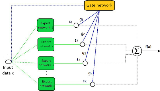
Our MoE architecture comprises expert networks responsible for handling specific features of the images. These experts work in parallel with a gating network, which learns to assign weights to each expert based on the input data. The collective decision made by the experts through the gating mechanism yields the final classification output.
One important aspect of building such a method is to select the right expert models artchitecture and select a good gating model too, Usually, this depends on the task itself. in this article, our experts will be simple convolutional neural networks while the gating model will be a simple feedforward network, to learn the gating weights.

1. Expert Networks:
Our MoE architecture comprises of 3 expert networks responsible for handling specific features of the images. For CIFAR-10, we design multiple expert networks, each specializing in recognizing distinctive patterns for a particular class. Convolutional layers and non-linear activation functions, such as ReLU, are used to capture hierarchical features.
2. Gating Network:
The gating network is important for selecting the most relevant expert for a given input. We employ a separate neural network, i.e., a simple feedforward network, to learn the gating weights. This network is trained concurrently with the expert networks to optimize the overall performance.
Training the Entire MoE
Training a MoE model involves optimizing both the expert networks and the gating network. We employ strategies such as layer-wise pre-training and curriculum learning to enhance convergence and stability. Regularization techniques, including dropout and weight decay, are applied to prevent overfitting.
during the training, the MoE model requires an iterative approach. in here, we will start by training expert networks independently and gradually introduce the gating network to fine-tune the interactions.
Implementing the MoE for CIFAR10 image Classification in TensorFlow
The code below shows the implementation of the experts, the gating model, the MoE, and finally the training process of the whole MoE model.
import tensorflow as tf
from tensorflow.keras import layers
from tensorflow.keras.layers.experimental import preprocessing
from keras.utils import to_categorical
import numpy as np
# Load the CIFAR-10 dataset
(x_train, y_train), (x_test, y_test) = tf.keras.datasets.cifar10.load_data()
# Normalize pixel values between 0 and 1
x_train = x_train.astype("float32") / 255
x_test = x_test.astype("float32") / 255
# Convert labels to one-hot encoding
num_classes = 10  # classes for images
y_train = to_categorical(y_train, num_classes)
y_test= to_categorical(y_test, num_classes)
from keras import layers, models
# Expert Model
def create_expert_model(input_shape, num_outputs):
    model = models.Sequential([
        layers.Conv2D(32, (3, 3), activation='relu', input_shape=input_shape),
        layers.MaxPooling2D((2, 2)),
        layers.Conv2D(64, (3, 3), activation='relu'),
        layers.MaxPooling2D((2, 2)),
        layers.Conv2D(128, (3, 3), activation='relu'),
        layers.MaxPooling2D((2, 2)),
        layers.Flatten(),
        layers.Dense(128, activation='relu'),
        layers.Dense(num_outputs, activation='softmax')
    ])
    return model
# Gating Model
def create_gating_model(num_experts, num_outputs):
    model = models.Sequential([
        layers.Dense(64, activation='relu', input_shape=(num_experts,)),
        layers.Dense(num_outputs, activation='softmax')
    ])
    return model
# Mixture of Experts (MOE) Model
def create_moe_model(input_shape, num_experts, num_outputs):
    expert_input = layers.Input(shape=input_shape, name='expert_input')
    expert_model = create_expert_model(input_shape, num_outputs)
    expert_output = expert_model(expert_input)
    gating_input = layers.Input(shape=(num_experts,), name='gating_input')
    gating_model = create_gating_model(num_experts, num_outputs)
    gating_output = gating_model(gating_input)
    # Reshape gating output to match expert output shape
    gating_output = layers.Reshape((num_outputs, 1))(gating_output)
    gating_output = layers.Lambda(lambda x: layers.Flatten()(x))(gating_output)
    # Multiply expert and gating outputs
    mixture_output = layers.Multiply()([expert_output, gating_output])
    moe_model = models.Model(inputs=[expert_input, gating_input], outputs=mixture_output)
    return moe_model
# Example usage:
input_shape = (32, 32, 3)  #
num_experts = 5  # Adjust based on the desired number of experts
num_outputs = 10  # Number of Cifar10 imageclasses
epochs = 30
moe_model = create_moe_model(input_shape, num_experts, num_outputs)
moe_model.compile(optimizer='adam', loss='categorical_crossentropy', metrics=['accuracy'])
#Train and Test
import matplotlib.pyplot as plt
history = moe_model.fit(
    [x_train, np.random.rand(len(x_train), num_experts)],
    y_train,
    epochs=epochs,
    batch_size=64)
plt.plot(history.history['loss'], label='Training Loss')
plt.plot(history.history['val_loss'], label='Validation Loss')
plt.xlabel('Epoch')
plt.ylabel('Loss')
plt.legend()
plt.show()
# Evaluate the model on the test set
test_loss, test_accuracy = moe_model.evaluate([x_test, np.random.rand(len(x_test), num_experts)], y_test_one_hot)
print(f'Test Accuracy: {test_accuracy * 100:.2f}%')
Results
Here is the learning process:
Epoch 1/35
782/782 [==============================] - 17s 21ms/step - loss: 1.5528 - accuracy: 0.4363
Epoch 2/35
782/782 [==============================] - 22s 28ms/step - loss: 1.1602 - accuracy: 0.5914
Epoch 3/35
782/782 [==============================] - 26s 34ms/step - loss: 1.0008 - accuracy: 0.6504
Epoch 4/35
782/782 [==============================] - 20s 25ms/step - loss: 0.8857 - accuracy: 0.6912
Epoch 5/35
782/782 [==============================] - 20s 25ms/step - loss: 0.7989 - accuracy: 0.7229
Epoch 6/35
782/782 [==============================] - 16s 21ms/step - loss: 0.7347 - accuracy: 0.7453
Epoch 7/35
782/782 [==============================] - 17s 22ms/step - loss: 0.6759 - accuracy: 0.7665
Epoch 8/35
782/782 [==============================] - 19s 25ms/step - loss: 0.6204 - accuracy: 0.7849
Epoch 9/35
782/782 [==============================] - 21s 27ms/step - loss: 0.5731 - accuracy: 0.7991
Epoch 10/35
782/782 [==============================] - 31s 39ms/step - loss: 0.5289 - accuracy: 0.8151
Epoch 11/35
782/782 [==============================] - 18s 23ms/step - loss: 0.4891 - accuracy: 0.8282
Epoch 12/35
782/782 [==============================] - 22s 29ms/step - loss: 0.4547 - accuracy: 0.8408
Epoch 13/35
782/782 [==============================] - 25s 32ms/step - loss: 0.4145 - accuracy: 0.8548
Epoch 14/35
782/782 [==============================] - 21s 27ms/step - loss: 0.3740 - accuracy: 0.8675
Epoch 15/35
782/782 [==============================] - 24s 30ms/step - loss: 0.3480 - accuracy: 0.8753
Epoch 16/35
782/782 [==============================] - 22s 28ms/step - loss: 0.3149 - accuracy: 0.8863
Epoch 17/35
782/782 [==============================] - 25s 32ms/step - loss: 0.2888 - accuracy: 0.8971
Epoch 18/35
782/782 [==============================] - 18s 23ms/step - loss: 0.2666 - accuracy: 0.9052
Epoch 19/35
782/782 [==============================] - 17s 21ms/step - loss: 0.2437 - accuracy: 0.9112
Epoch 20/35
782/782 [==============================] - 18s 23ms/step - loss: 0.2219 - accuracy: 0.9208
Epoch 21/35
782/782 [==============================] - 20s 26ms/step - loss: 0.1963 - accuracy: 0.9286
Epoch 22/35
782/782 [==============================] - 22s 28ms/step - loss: 0.1874 - accuracy: 0.9329
Epoch 23/35
782/782 [==============================] - 23s 30ms/step - loss: 0.1712 - accuracy: 0.9387
Epoch 24/35
782/782 [==============================] - 20s 26ms/step - loss: 0.1580 - accuracy: 0.9440
Epoch 25/35
782/782 [==============================] - 20s 25ms/step - loss: 0.1537 - accuracy: 0.9444
Epoch 26/35
782/782 [==============================] - 17s 22ms/step - loss: 0.1370 - accuracy: 0.9500
Epoch 27/35
782/782 [==============================] - 21s 27ms/step - loss: 0.1380 - accuracy: 0.9506
Epoch 28/35
782/782 [==============================] - 17s 22ms/step - loss: 0.1339 - accuracy: 0.9520
Epoch 29/35
782/782 [==============================] - 17s 22ms/step - loss: 0.1068 - accuracy: 0.9615
Epoch 30/35
782/782 [==============================] - 20s 26ms/step - loss: 0.1191 - accuracy: 0.9579
Epoch 31/35
782/782 [==============================] - 17s 22ms/step - loss: 0.1194 - accuracy: 0.9574
Epoch 32/35
782/782 [==============================] - 20s 25ms/step - loss: 0.1006 - accuracy: 0.9643
Epoch 33/35
782/782 [==============================] - 18s 23ms/step - loss: 0.1136 - accuracy: 0.9599
Epoch 34/35
782/782 [==============================] - 18s 23ms/step - loss: 0.1031 - accuracy: 0.9634
Epoch 35/35
782/782 [==============================] - 18s 23ms/step - loss: 0.1026 - accuracy: 0.9646
313/313 [==============================] - 2s 5ms/step - loss: 1.9688 - accuracy: 0.7066
Test Accuracy: 70.66%
If you like the article and would like to support me make sure to:
📰 View more content on my medium profile and
👏Clap for this article
📰 View more content on AI-ContentLab Blog
🚀👉 Read more related articles to this one on Medium and AI-ContentLab
Comments
Post a Comment