Knee Osteoarthritis Diagnosis: A Deep Learning Approach with Mixture of Experts

 Osteoarthritis (OA) of the knee is a degenerative condition affecting three knee compartments (lateral, medial, and patella-femoral), typically developing gradually over a span of 10 to 15 years [1,2]. Primarily caused by wear, tear, and progressive loss of articular cartilage, it can also result from infections leading to joint cavity damage, resulting in discomforts such as limited mobility, joint pain, and swelling [3]. Cartilage tissue alterations and damage are common in all joints, with the knee and hip joints being particularly susceptible due to their weight-bearing nature. Knee OA predominantly occurs in individuals aged over 55, with a higher prevalence among those over 65, and it is estimated that by 2050, 130 million individuals globally will be affected. Early detection and treatment are crucial for mitigating the progression of knee OA and enhancing individuals' quality of life [5].

The complexity of diagnosing and treating knee OA lies in its multifaceted nature, with numerous risk factors involved, including advanced age, gender, hormonal status, and body mass index (BMI). Additionally, various medical, environmental, and biological factors contribute to the disease's development and progression, both modifiable and non-modifiable. In severe cases, patients with these risk factors may undergo total knee replacement. Presently, behavioral interventions such as weight loss, physical exercise, and joint muscle strengthening represent the primary therapies for individuals with knee OA. While these interventions may offer temporary pain relief and slow disease progression, there is a pressing need for more effective treatment options [6,7].

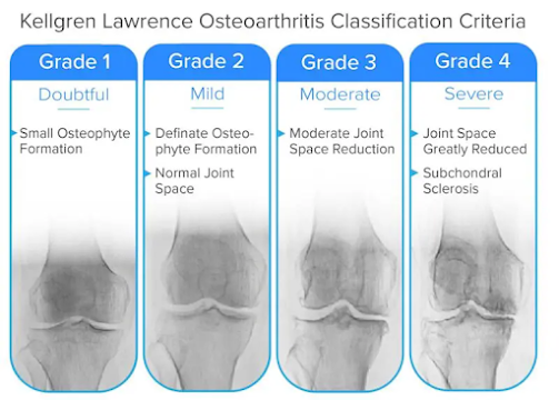
Accurate grading of knee OA is crucial for effective treatment planning and monitoring disease progression. Traditional grading systems often lack the precision required for personalized care, prompting researchers to explore advanced techniques. 

In previous articles, we discussed  Mixtures of Experts and provided a review of Knee Osteoarthritis using deep learning. 

In this blog post, we delve into the complexities of knee OA grading, review the latest works in the field, discuss the challenges faced, and propose an innovative solution using Mixture of Experts (MoE) implemented with TensorFlow.

                                                                                                Source

Review of Latest Works:

Several recent studies have explored machine learning (ML) and deep learning (DL) approaches to improve knee OA grading accuracy. Convolutional Neural Networks (CNNs) have shown promise in image-based grading, but challenges persist, including the need for large labeled datasets and interpretability issues. Transfer learning and ensemble methods have also been explored, providing incremental improvements.

Antony et al. [7] proposed a new method to quantify the severity of knee osteoarthritis (OA) based on X-ray images. They used KL grades as training input to train a fully convolutional neural network (FCNN) to quantify knee OA severity. Data from the Osteoarthritis Initiative (OAI) and Multicenter Osteoarthritis Study (MOST) were utilized to appraise the effectiveness of this model. The empirical results of this method were compared to previously existing methods, and improvements in classification accuracy, recall, F1 score, and precision were observed.

Norman et al. [8] proposed a novel approach for the assessment of OA in knee X-rays based on KL grading. Their approach uses state-of-the-art neural networks to implement ensemble learning for precise classification from raw X-ray images. They stated that their approach might be utilized to benefit radiologists in making a quite reliable diagnosis.

Tiulpin et al. [9] suggested an automated diagnostic technique based on deep Siamese convolutional neural networks (CNNs), which acquire a similarity measure between images. This concept is not limited to simple image pair comparisons but is instead used to compare knee X-rays (with symmetrical joints). Particularly, this network can learn identical weights for both knee joints if the images are split at the central location and fed to a separate CNN branch. Simulation results on the entire OAI dataset demonstrated that their work outperforms previous models, with an accuracy score of 66.71%.

Chen et al. [1] employed two CNNs to grade knee OA severity based on the KL grading system. A specialized one-stage YOLOv2 network was used to detect X-ray images of knee joints. Using the best-performing CNNs, including versions of YOLO, ResNet, VGG, DenseNet, and InceptionV3, the detected knee joint images were then classified utilizing adjusted ordinal loss analysis. Empirical results revealed that the best classification accuracy and the mean absolute error obtained with their proposed approach are 69.7% and 0.344, respectively.

Understanding the Problem:

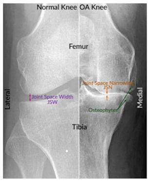
Knee OA grading involves assessing the severity of cartilage degradation, joint space narrowing, and osteophyte formation. Traditional methods rely on radiographic imaging, but the subjective nature of visual grading and the nuances of disease presentation make it a challenging task. Achieving consistent and accurate grading is essential for guiding treatment decisions.

                                                                              Source

Challenges in Knee OA Grading:

• Limited Labeled Data: Building robust models requires large, diverse, and accurately labeled datasets, which are often scarce in the medical domain.
• Inter-Observer Variability: Different clinicians may interpret the same radiographic images differently, leading to inconsistencies in grading.
• Non-Linearity in Disease Progression: Knee OA is a complex, nonlinear condition with variations in disease manifestation, making it challenging to capture using traditional linear models.
• Interpretability and Explainability: Understanding the decisions of AI models is crucial in medical applications. Ensuring that the model's predictions align with clinical reasoning is essential for widespread adoption.

Proposed Solution: Mixture of Experts 

Mixture of Experts (MoE) is a neural network architecture that combines the strengths of both global and local models. It consists of expert networks responsible for specific regions of the input space and a gating network that determines the contribution of each expert to the final prediction. This approach enables capturing the intricate patterns present in knee OA images.

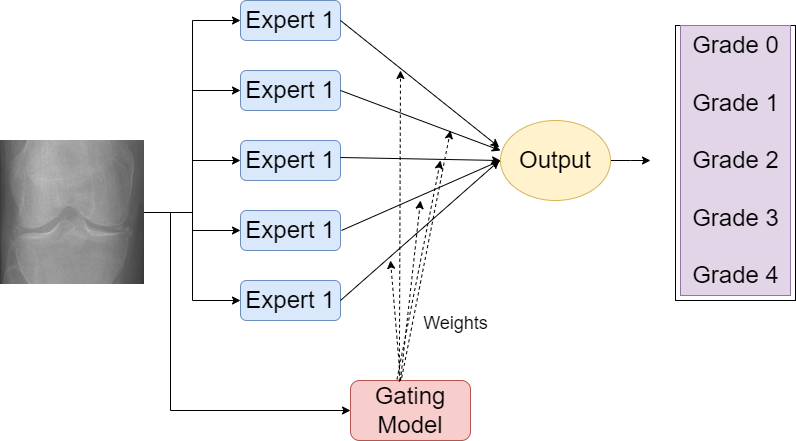
Proposed Framework for KOA Grading Using MoE. Drawn by Author

Implementation Steps:

• Data Preprocessing:

1. Load and preprocess knee OA radiographic images.
2. Split the dataset into training, validation, and test sets.

• Model Architecture:

1. Design the MoE architecture using TensorFlow or PyTorch.
2. Define expert networks and a gating network.
3. Train the model on the training dataset.

• Training Strategy:

1. Employ techniques like data augmentation to enhance model generalization.
2. Implement transfer learning if pre-trained models are available.

• Evaluation:

1. Assess the model on the validation set and fine-tune hyperparameters.
2. Evaluate the final model on the test set to measure its performance.

• Interpretability:

1. Implement methods to interpret and explain the decisions made by the MoE model.

Implementation of Mixture of Experts for Knee Osteoarthritis Grading in TensorFlow

Implementing the proposed solution involves several steps, including data preprocessing, model architecture design, training strategy, evaluation, and interpretability. Below is a simplified code outline using TensorFlow. Note that this is a high-level representation, and additional optimizations and fine-tuning may be required for practical implementation based on specific data characteristics.

First, we load the data. we get the X-ray knee radiographs from the OAI dataset. 

import os

import cv2

import numpy as np

from sklearn.model_selection import train_test_split

from keras.utils import to_categorical



# Function to load and preprocess knee OA radiographic images

def load_and_preprocess_data(base_dir, image_size=(64, 64)):

    data = []

    labels = []



    # Iterate through subdirectories (each subdirectory corresponds to a class)

    for class_label in os.listdir(base_dir):

        class_path = os.path.join(base_dir, class_label)

        

        for image_file in os.listdir(class_path):

            image_path = os.path.join(class_path, image_file)

            

            # Read and resize the image

            image = cv2.imread(image_path)

            image = cv2.resize(image, image_size)

            

            # Normalize pixel values to be between 0 and 1

            image = image.astype('float32') / 255.0



            data.append(image)

            labels.append(int(class_label))  # Assuming subdirectory names represent class labels



    return np.array(data), np.array(labels)



# Load and preprocess knee OA radiographic images

base_dir = r'C:\Users\abdul\Desktop\Research\Knee Osteo\56rmx5bjcr-1\KneeXrayData\KneeXrayData\ClsKLData\kneeKL224'

data, labels = load_and_preprocess_data(base_dir)



# Split the dataset into training, validation, and test sets

X_train, X_temp, y_train, y_temp = train_test_split(data, labels, test_size=0.3, random_state=42)

X_val, X_test, y_val, y_test = train_test_split(X_temp, y_temp, test_size=0.5, random_state=42)



# Convert labels to one-hot encoding

num_classes = 5  # Assuming 5 classes for KOA grading

y_train_one_hot = to_categorical(y_train, num_classes)

y_val_one_hot = to_categorical(y_val, num_classes)

y_test_one_hot = to_categorical(y_test, num_classes)

Now that, the data is loaded, let's start creating our Expert models architecture. we will use a CNN-based model.  The expert model used here is a convolutional neural network (CNN) responsible for processing a specific region of the input data. In this case, it's designed as a simple CNN with convolutional layers followed by max-pooling and dense layers. This structure is meant for learning hierarchical features from knee OA radiographic images.

# Expert Model

def create_expert_model(input_shape, num_outputs):

    model = models.Sequential([

        layers.Conv2D(32, (3, 3), activation='relu', input_shape=input_shape),

        layers.MaxPooling2D((2, 2)),

        layers.Conv2D(64, (3, 3), activation='relu'),

        layers.MaxPooling2D((2, 2)),

        layers.Conv2D(128, (3, 3), activation='relu'),

        layers.MaxPooling2D((2, 2)),

        layers.Flatten(),

        layers.Dense(128, activation='relu'),

        layers.Dense(num_outputs, activation='softmax')

    ])

    return model

The next step is to create the Gating model. The gating model used here is a neural network responsible for determining the contribution of each expert to the final prediction. It takes the same input shape as the expert model but outputs probabilities assigned to each expert using a softmax activation function.

# Gating Model

def create_gating_model(num_experts, num_outputs):

    model = models.Sequential([

        layers.Dense(128, activation='relu', input_shape=(num_experts,)),

        layers.Dense(num_outputs, activation='softmax')

    ])

    return model

That done, let's create the Mixture. The Mixture of Experts (MoE) model combines the expert and gating models. It takes two inputs: one for the expert model and one for the gating model. The Multiply layer is used to weight the expert outputs based on the probabilities determined by the gating model.

# Mixture of Experts (MOE) Model

def create_moe_model(input_shape, num_experts, num_outputs):

    expert_input = layers.Input(shape=input_shape, name='expert_input')

    expert_model = create_expert_model(input_shape, num_outputs)

    expert_output = expert_model(expert_input)

    gating_input = layers.Input(shape=(num_experts,), name='gating_input')

    gating_model = create_gating_model(num_experts, num_outputs)

    gating_output = gating_model(gating_input)



    # Reshape gating output to match expert output shape

    gating_output = layers.Reshape((num_outputs, 1))(gating_output)

    gating_output = layers.Lambda(lambda x: layers.Flatten()(x))(gating_output)



    # Multiply expert and gating outputs

    mixture_output = layers.Multiply()([expert_output, gating_output])

    moe_model = models.Model(inputs=[expert_input, gating_input], outputs=mixture_output)

    return moe_model

Training Strategy:

The MoE model is compiled using the Adam optimizer and binary cross-entropy loss since it's a binary classification problem (KOA grading, 5 grades). The training strategy involves using an ImageDataGenerator for data augmentation, and the model is trained using the fit method.

# Assuming you have already defined the create_moe_model function from the previous response

# Specify input shape, number of experts, and number of classes
input_shape = (64, 64, 1)  # Input image dimensions
num_experts = 5  #  number of experts
num_classes = 5  # Number of KOA grading classes

# Create the Mixture of Experts (MOE) model
moe_model = create_moe_model(input_shape, num_experts, num_classes)

# Compile the model
moe_model.compile(optimizer='adam', loss='categorical_crossentropy', metrics=['accuracy'])

# Train the model
epochs = 20
batch_size = 32

history = moe_model.fit(
    [X_train, np.random.rand(len(X_train), num_experts)],
    y_train_one_hot,
    epochs=epochs,
    batch_size=batch_size,
    validation_data=([X_val, np.random.rand(len(X_val), num_experts)], y_val_one_hot)
)

# Evaluate the model on the test set
test_loss, test_accuracy = moe_model.evaluate([X_test, np.random.rand(len(X_test), num_experts)], y_test_one_hot)

print(f'Test Accuracy: {test_accuracy * 100:.2f}%')

Loss Function:

The binary cross-entropy loss is commonly used for binary classification problems. It measures the difference between the predicted probabilities and the true labels. In this case, the MoE model aims to minimize this loss during training.

The training process involves optimizing the parameters of both the expert and gating models jointly to minimize this loss function, creating a model that accurately predicts knee osteoarthritis severity based on radiographic images.

The use of [X_train, np.random.rand(len(X_train), num_experts)] in the context of training the MoE corresponds to providing two inputs to our model during training. Let's break it down:

• X_train: This is our actual input data, presumably the knee osteoarthritis radiographic images.
• np.random.rand(len(X_train), num_experts): This is a random array generated using NumPy. It creates an array with a shape of (len(X_train), num_experts). This array is used as additional input, typically for the gating network in the mixture-of-experts model.

In the mixture-of-experts model, the gating network learns to assign weights to different experts based on the input data. The random array is often used as an auxiliary input to the gating network during training. This can introduce some level of noise or exploration, which might be beneficial for training the model, especially if the training is challenging.

So, during each training iteration, our model receives two inputs: the actual data (X_train) and a random array (np.random.rand(len(X_train), num_experts)), which is intended to provide some form of randomization or exploration in the training process. This is a common strategy in mixture-of-experts models to help the model generalize better and prevent overfitting.

Training and Evaluation

we ran the code for 20 epochs where 5 experts were used and here are the results: 

Epoch 1/20
157/157 [==============================] - 12s 73ms/step - loss: 1.4890 - accuracy: 0.3559 - val_loss: 1.4881 - val_accuracy: 0.3684
Epoch 2/20
157/157 [==============================] - 11s 70ms/step - loss: 1.4773 - accuracy: 0.3591 - val_loss: 1.4840 - val_accuracy: 0.3684
Epoch 3/20
157/157 [==============================] - 8s 50ms/step - loss: 1.4614 - accuracy: 0.3608 - val_loss: 1.4230 - val_accuracy: 0.3721
Epoch 4/20
157/157 [==============================] - 11s 70ms/step - loss: 1.3706 - accuracy: 0.3838 - val_loss: 1.3056 - val_accuracy: 0.4260
Epoch 5/20
157/157 [==============================] - 9s 57ms/step - loss: 1.2741 - accuracy: 0.4222 - val_loss: 1.2533 - val_accuracy: 0.4567
Epoch 6/20
157/157 [==============================] - 10s 64ms/step - loss: 1.2253 - accuracy: 0.4492 - val_loss: 1.2030 - val_accuracy: 0.4679
Epoch 7/20
157/157 [==============================] - 11s 70ms/step - loss: 1.1856 - accuracy: 0.4661 - val_loss: 1.2973 - val_accuracy: 0.3777
Epoch 8/20
157/157 [==============================] - 9s 57ms/step - loss: 1.1566 - accuracy: 0.4821 - val_loss: 1.1579 - val_accuracy: 0.4930
Epoch 9/20
157/157 [==============================] - 12s 74ms/step - loss: 1.1304 - accuracy: 0.4880 - val_loss: 1.1321 - val_accuracy: 0.4940
Epoch 10/20
157/157 [==============================] - 11s 71ms/step - loss: 1.1121 - accuracy: 0.5040 - val_loss: 1.1053 - val_accuracy: 0.5107
Epoch 11/20
157/157 [==============================] - 11s 69ms/step - loss: 1.0854 - accuracy: 0.5163 - val_loss: 1.1183 - val_accuracy: 0.5033
Epoch 12/20
157/157 [==============================] - 11s 71ms/step - loss: 1.0756 - accuracy: 0.5148 - val_loss: 1.1826 - val_accuracy: 0.4735
Epoch 13/20
157/157 [==============================] - 12s 75ms/step - loss: 1.0611 - accuracy: 0.5249 - val_loss: 1.0969 - val_accuracy: 0.5107
Epoch 14/20
157/157 [==============================] - 8s 52ms/step - loss: 1.0345 - accuracy: 0.5373 - val_loss: 1.1147 - val_accuracy: 0.4995
Epoch 15/20
157/157 [==============================] - 11s 67ms/step - loss: 1.0219 - accuracy: 0.5441 - val_loss: 1.1329 - val_accuracy: 0.5228
Epoch 16/20
157/157 [==============================] - 10s 61ms/step - loss: 1.0286 - accuracy: 0.5419 - val_loss: 1.1324 - val_accuracy: 0.4223
Epoch 17/20
157/157 [==============================] - 9s 60ms/step - loss: 1.0015 - accuracy: 0.5486 - val_loss: 1.0764 - val_accuracy: 0.5144
Epoch 18/20
157/157 [==============================] - 13s 82ms/step - loss: 0.9814 - accuracy: 0.5590 - val_loss: 1.0627 - val_accuracy: 0.5293
Epoch 19/20
157/157 [==============================] - 10s 61ms/step - loss: 0.9768 - accuracy: 0.5702 - val_loss: 1.1044 - val_accuracy: 0.5126
Epoch 20/20
157/157 [==============================] - 8s 52ms/step - loss: 0.9527 - accuracy: 0.5712 - val_loss: 1.0604 - val_accuracy: 0.5200
34/34 [==============================] - 1s 15ms/step - loss: 1.0263 - accuracy: 0.5428
Test Accuracy: 54.28%

The Learning and Loss curve

import matplotlib.pyplot as plt
plt.plot(history.history['loss'], label='Training Loss')
plt.plot(history.history['val_loss'], label='Validation Loss')
plt.xlabel('Epoch')
plt.ylabel('Loss')
plt.legend()
plt.show()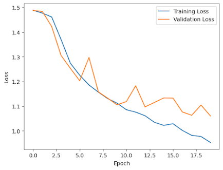

Model Explainability Using Grad-Cam 

To visualize the model's learned activation maps using Grad-CAM (Gradient-weighted Class Activation Mapping), you can follow these general steps:

import tensorflow as tf
import numpy as np
import cv2
from matplotlib import pyplot as plt

def preprocess_image(img_path):
    img = tf.keras.preprocessing.image.load_img(img_path, target_size=(224, 224))
    img_array = tf.keras.preprocessing.image.img_to_array(img)
    img_array = np.expand_dims(img_array, axis=0)
    img_array = tf.keras.applications.mobilenet_v2.preprocess_input(img_array)
    return img_array

def get_grad_cam(model, img_array, layer_name):
    grad_model = tf.keras.models.Model(
        [model.inputs], [model.get_layer(layer_name).output, model.output]
    )

    with tf.GradientTape() as tape:
        conv_outputs, predictions = grad_model(img_array)
        loss = predictions[:, np.argmax(predictions[0])]

    grads = tape.gradient(loss, conv_outputs)[0]
    guided_grads = tf.cast(conv_outputs > 0, 'float32') * tf.cast(grads > 0, 'float32') * grads

    weights = tf.reduce_mean(guided_grads, axis=(0, 1))
    cam = tf.reduce_sum(tf.multiply(weights, conv_outputs), axis=-1)
    
    return cam.numpy()

def overlay_grad_cam(img_path, cam, alpha=0.4):
    img = cv2.imread(img_path)
    img = cv2.resize(img, (224, 224))

    heatmap = cv2.resize(cam, (img.shape[1], img.shape[0]))
    heatmap = np.uint8(255 * heatmap)
    heatmap = cv2.applyColorMap(heatmap, cv2.COLORMAP_JET)

    superimposed_img = cv2.addWeighted(img, alpha, heatmap, 1 - alpha, 0)

    return superimposed_img

# Load the trained model
model = tf.keras.models.load_model('your_model_path.h5')

# Load and preprocess the image
img_path = 'image1.jpg'
img_array = preprocess_image(img_path)

# Choose the layer for which you want to visualize the activation map
layer_name = 'Conv1'

# Get the Grad-CAM
cam = get_grad_cam(model, img_array, layer_name)

# Overlay Grad-CAM on the original image and display
result = overlay_grad_cam(img_path, cam)
plt.imshow(result)
plt.axis('off')
plt.show()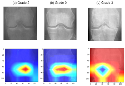

Summary

In this post, we focused on building and training a model for Knee Osteoarthritis (KOA) grading, a multi-class classification problem with five classes. We designed a Mixture of Experts (MOE) model, consisting of an expert model for image feature extraction, a gating model for attention, and a combination of these using the Mixture of Experts approach. Ofcourse, this is just a simple framework but to achieve better results you need more complex MoE, and you need to try different architectures for the experts and Gating model. 

If you like the article and would like to support me make sure to:
📰 View more content on AI-ContentLab Blog 
📰 View more content on my medium profile
🔔 Follow Me: LinkedIn | Medium | GitHub | Facebook
🚀👉 Read more related articles to this one on Medium and AI-ContentLab

References

[1] Chen, P.; Gao, L.; Shi, X.; Allen, K.; Yang, L. Fully Automatic Knee Osteoarthritis Severity Grading Using Deep Neural Networks with a Novel Ordinal Loss. Comput. Med. Imaging Graph. 2019, 75, 84–92. 

[2] Kim, D.H.; Kim, S.C.; Yoon, J.S.; Lee, Y.S. Are There Harmful Effects of Preoperative Mild Lateral or Patellofemoral Degeneration on the Outcomes of Open Wedge High Tibial Osteotomy for Medial Compartmental Osteoarthritis? Orthop. J. Sport. Med. 2020, 8, 2325967120927481. [Google Scholar] 

[3] Tiulpin, A.; Saarakkala, S. Automatic Grading of Individual Knee Osteoarthritis Features in Plain Radiographs Using Deep Convolutional Neural Networks. Diagnostics 2020, 10, 932.

[4] Postler, A.; Luque Ramos, A.; Goronzy, J.; Günther, K.P.; Lange, T.; Schmitt, J.; Zink, A.; Hoffmann, F. Prevalence and Treatment of Hip and Knee Osteoarthritis in People Aged 60 Years or Older in Germany: An Analysis Based on Health Insurance Claims Data. Clin. Interv. Aging 2018, 13, 2339–2349.

[5] Wang, Y.; Wang, X.; Gao, T.; Du, L.; Liu, W. An Automatic Knee Osteoarthritis Diagnosis Method Based on Deep Learning: Data from the Osteoarthritis Initiative. J. Healthc. Eng. 2021, 2021, 5586529. 

[6] Roos, E.M.; Arden, N.K. Strategies for the Prevention of Knee Osteoarthritis. Nat. Rev. Rheumatol. 2016, 12, 92–101. 

[7] Antony, J.; McGuinness, K.; Moran, K.; O’Connor, N.E. Automatic Detection of Knee Joints and Quantification of Knee Osteoarthritis Severity Using Convolutional Neural Networks. In International Conference on Machine Learning and Data Mining in Pattern Recognition; Springer: Berlin/Heidelberg, Germany, 2017; pp. 376–390. [Google Scholar]

[8] Norman, B.; Pedoia, V.; Noworolski, A.; Link, T.M.; Majumdar, S. Applying Densely Connected Convolutional Neural Networks for Staging Osteoarthritis Severity from Plain Radiographs. J. Digit. Imaging 2019, 32, 471–477. [Google Scholar] [CrossRef] [PubMed]

[9] Tiulpin, A.; Thevenot, J.; Rahtu, E.; Lehenkari, P.; Saarakkala, S. Automatic Knee Osteoarthritis Diagnosis from Plain Radiographs: A Deep Learning-Based Approach. Sci. Rep. 2018, 8, 1727. [Google Scholar] [CrossRef][Green Version]

[10] Moustakidis, S.; Papandrianos, N.I.; Christodolou, E.; Papageorgiou, E.; Tsaopoulos, D. Dense Neural Networks in Knee Osteoarthritis Classification: A Study on Accuracy and Fairness. Neural Comput. Appl. 2020, 5, 1–13. [Google Scholar] [CrossRef]

[11] Thomas, K.A.; Kidziński, Ł.; Halilaj, E.; Fleming, S.L.; Venkataraman, G.R.; Oei, E.H.G.; Gold, G.E.; Delp, S.L. Automated Classification of Radiographic Knee Osteoarthritis Severity Using Deep Neural Networks. Radiol. Artif. Intell. 2020, 2, e190065. [Google Scholar] [CrossRef] [PubMed]