Deep learning is a branch of machine learning that uses artificial neural networks to perform complex calculations on large datasets. It mimics the structure and function of the human brain and trains machines by learning from examples. Deep learning is widely used by industries that deal with complex problems, such as health care, eCommerce, entertainment, and advertising.
This post explores the basic types of artificial neural networks and how they work to enable deep learning algorithms.
Defining Neural Networks
A neural network is modeled after the human brain and has artificial neurons or nodes. These nodes are arranged in three layers:
- The input layer
- The hidden layer(s)
- The output layer
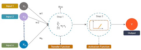
The input layer feeds each node with data as inputs. The node then applies random weights, a bias, and a nonlinear function, also called an activation function, to the inputs. The activation function decides which neuron to activate.
How Deep Learning Works!
Deep learning is a type of machine learning that uses artificial neural networks to perform sophisticated computations on large amounts of data. It works based on the structure and function of the human brain and trains machines by learning from examples. Deep learning algorithms rely on ANNs that simulate how the brain processes information. They use unknown factors in the input data to learn features, group objects, and find useful patterns in the data. They train machines to learn by themselves at different levels, using the algorithms to create the models.
Some of the basics of deep learning and lists the top 10 most popular deep learning algorithms. These algorithms are:
- Convolutional Neural Networks (CNNs): These are neural networks that use convolutional layers to extract features from images, videos, or other types of data. They are widely used for image recognition, face detection, natural language processing, and computer vision tasks.
- Long Short Term Memory Networks (LSTMs): These are a type of recurrent neural networks that can remember long-term dependencies and sequences of data. They are useful for natural language processing, speech recognition, text generation, and time series analysis.
- Recurrent Neural Networks (RNNs): These are neural networks that have loops that allow them to process sequential data. They can learn from previous inputs and outputs and generate predictions based on the context. They are used for natural language processing, speech recognition, text generation, and time series analysis.
- Generative Adversarial Networks (GANs): These are neural networks that consist of two competing models: a generator and a discriminator. The generator tries to create realistic data that can fool the discriminator, while the discriminator tries to distinguish between real and fake data. They are used for image synthesis, image editing, style transfer, and data augmentation.
- Radial Basis Function Networks (RBFNs): These are neural networks that use radial basis functions as activation functions. They can approximate any continuous function and are good for interpolation, regression, and classification tasks.
- Multilayer Perceptrons (MLPs): These are the simplest type of neural networks that consist of multiple layers of nodes connected by weights. They can learn nonlinear functions and are used for classification, regression, and function approximation tasks.
- Self Organizing Maps (SOMs): These are neural networks that use unsupervised learning to create a low-dimensional representation of high-dimensional data. They can cluster data, visualize data, and perform dimensionality reduction.
- Deep Belief Networks (DBNs): These are neural networks that are composed of multiple layers of restricted Boltzmann machines. They can learn complex patterns and features from unlabeled data and are used for feature extraction, dimensionality reduction, and generative modeling.
- Restricted Boltzmann Machines (RBMs): These are neural networks that have two layers: a visible layer and a hidden layer. They can learn the probability distribution of the input data and are used for feature extraction, dimensionality reduction, and generative modeling.
- Autoencoders: These are neural networks that learn to encode the input data into a lower-dimensional representation and then decode it back to the original data. They can learn useful features, compress data, and perform denoising, anomaly detection, and generative modeling.
These algorithms can be applied to various cybersecurity problems, such as threat detection, anomaly recognition, and predictive analysis. For example, CNNs can be used to detect malicious images or files, LSTMs can be used to analyze network traffic or user behavior, and GANs can be used to generate synthetic data or adversarial examples.
Going Deep into Deep Networks
1. Convolutional Neural Networks (CNNs)
CNNs, or ConvNets, are neural networks that have multiple layers and are mainly used for image processing and object detection. They were first developed by Yann LeCun in 1988 and were called LeNet. They were used to recognize characters like digits and ZIP codes. CNNs are widely used to identify images from satellites, process images from medicine, predict time series, and detect anomalies.
CNNs work by having multiple layers that process and extract features from data:
- Convolution Layer: This layer has several filters that perform the convolution operation on the data.
- Rectified Linear Unit (ReLU): This layer applies a function to the elements of the data. The output is a rectified feature map.
- Pooling Layer: This layer reduces the dimensions of the feature map by performing a down-sampling operation.
- The pooling layer then flattens the resulting two-dimensional arrays from the pooled feature map into a single, long, continuous, linear vector.
- Fully Connected Layer: This layer takes the flattened vector as an input and classifies and identifies the data.
The following is an example of an image processed by a CNN.

2. Long Short Term Memory Networks (LSTMs)
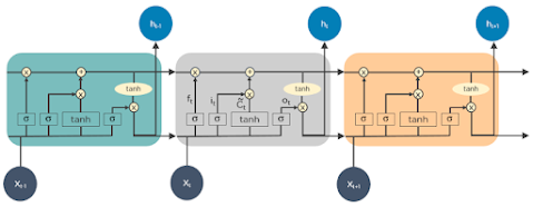
LSTMs are a kind of RNN that can learn and remember long-term dependencies. They can recall past information for long periods by default.
LSTMs keep information over time. They are useful for predicting time-series because they remember previous inputs. LSTMs have a chain-like structure where four layers interact in a special way. Besides predicting time-series, LSTMs are also used for speech recognition, music composition, and pharmaceutical development.
LSTMs work by following these steps:
- First, they forget irrelevant parts of the previous state
- Next, they selectively update the cell-state values
- Finally, they output certain parts of the cell state
The following is a diagram of how LSTMs operate:
3. Recurrent Neural Networks (RNNs)
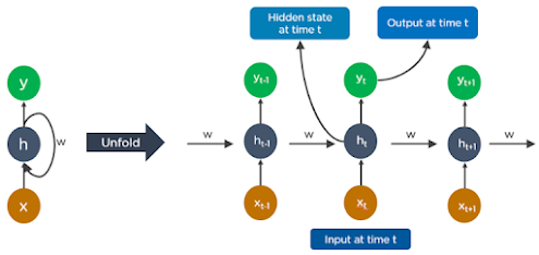
RNNs have connections that form loops, which allow the outputs from the LSTM to be used as inputs to the current phase.
The output from the LSTM becomes an input to the current phase and can remember previous inputs because of its internal memory. RNNs are widely used for image captioning, time-series analysis, natural-language processing, handwriting recognition, and machine translation. RNNs work by following these steps:
- The output at time t-1 is used as an input at time t.
- Similarly, the output at time t is used as an input at time t+1.
- RNNs can handle inputs of any length.
- The computation takes into account historical information, and the model size does not depend on the input size.
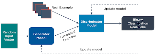
GANs are generative deep learning algorithms that create new data instances that look like the training data. GAN has two components: a generator, which learns to make fake data, and a discriminator, which learns from that false data.
GANs have become more popular over time. They can be used to enhance astronomical images and simulate gravitational lensing for dark-matter research. Video game developers use GANs to improve low-resolution, 2D textures in old video games by recreating them in 4K or higher resolutions using image training.
GANs can generate realistic images and cartoon characters, create photos of human faces, and render 3D objects.
GANs work by following these steps:
- The discriminator learns to tell the difference between the generator's fake data and the real sample data.
- In the beginning of the training, the generator makes fake data, and the discriminator easily learns to recognize that it's fake.
- The GAN sends the results to the generator and the discriminator to update the model.
The following is a diagram of how GANs operate:
5. Multilayer Perceptrons (MLPs)
MLPs are a good way to start learning about deep learning technology.
MLPs are a type of feedforward neural network with multiple layers of perceptrons that have activation functions. MLPs have an input layer and an output layer that are fully connected. They have the same number of input and output layers but can have multiple hidden layers. They can be used to build software for speech-recognition, image-recognition, and machine-translation.
MLPs work by following these steps:
- MLPs send the data to the input layer of the network. The layers of neurons connect in a graph so that the signal goes in one direction.
- MLPs calculate the input with the weights that exist between the input layer and the hidden layers.
- MLPs use activation functions to decide which nodes to activate. Activation functions include ReLUs, sigmoid functions, and tanh.
- MLPs train the model to understand the relationship and learn the dependencies between the independent and the target variables from a training data set.
The following is an example of an MLP. The diagram shows how weights and bias are computed and how activation functions are applied to classify images of cats and dogs.
6. Self Organizing Maps (SOMs)
SOMs are a type of artificial neural network that enables data visualization to reduce the dimensions of data through self-organizing. They were invented by Professor Teuvo Kohonen.
Data visualization tries to solve the problem that humans cannot easily see high-dimensional data. SOMs are made to help users understand this high-dimensional data.
SOMs work by following these steps:
- SOMs assign weights for each node and pick a random vector from the training data.
- SOMs check every node to find which weights are the closest to the input vector. The winning node is called the Best Matching Unit (BMU).
- SOMs find the neighbors of the BMU, and the number of neighbors decreases over time.
- SOMs update the winning weight to match the sample vector. The nearer a node is to the BMU, the more its weight changes.
- The farther the neighbor is from the BMU, the less it learns. SOMs repeat step two for N iterations.
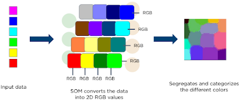
The following is a diagram of an input vector of different colors. This data goes to a SOM, which then transforms the data into 2D RGB values. Finally, it separates and groups the different colors.
7. Deep Belief Networks (DBNs)
DBNs are generative models that have multiple layers of random, hidden variables. The hidden variables have binary values and are also called hidden units.
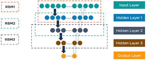
DBNs are a stack of Boltzmann Machines with connections between the layers, and each RBM layer communicates with both the previous and subsequent layers. DBNs are used for image-recognition, video-recognition, and motion-capture data.
DBNs work by following these steps:
- Greedy learning algorithms train DBNs. The greedy learning algorithm uses a layer-by-layer method for learning the top-down, generative weights.
- DBNs run the steps of Gibbs sampling on the top two hidden layers. This stage draws a sample from the RBM defined by the top two hidden layers.
- DBNs draw a sample from the visible units using a single pass of ancestral sampling through the rest of the model.
- DBNs learn that the values of the hidden variables in every layer can be inferred by a single, bottom-up pass.
The following is an example of DBN architecture:
8. Restricted Boltzmann Machines (RBMs)
RBMs are random neural networks that can learn from a probability distribution over a set of inputs. They were developed by Geoffrey Hinton and are used for dimensionality reduction, classification, regression, collaborative filtering, feature learning, and topic modeling. RBMs are the building blocks of DBNs.
RBMs have two layers:
- Visible units
- Hidden units
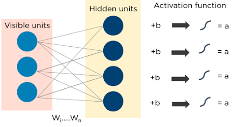
Each visible unit is connected to all hidden units. RBMs have a bias unit that is connected to all the visible units and the hidden units, and they have no output nodes.
RBMs work by following these steps:
- RBMs have two phases: forward pass and backward pass.
- RBMs take the inputs and convert them into a set of numbers that represents the inputs in the forward pass.
- RBMs combine each input with individual weight and one overall bias. The algorithm sends the output to the hidden layer.
- In the backward pass, RBMs take that set of numbers and convert them back to form the reconstructed inputs.
- RBMs combine each activation with individual weight and overall bias and send the output to the visible layer for reconstruction.
- At the visible layer, the RBM compares the reconstruction with the original input to measure the quality of the result.
The following is a diagram of how RBMs work:
9. Autoencoders
Autoencoders are a type of feedforward neural network that have the same input and output. They were designed by Geoffrey Hinton in the 1980s to solve unsupervised learning problems. They are trained neural networks that copy the data from the input layer to the output layer. Autoencoders are used for purposes such as pharmaceutical discovery, popularity prediction, and image processing.
Autoencoders have three main components: the encoder, the code, and the decoder.
Autoencoders are structured to take an input and change it into a different representation. They then try to reconstruct the original input as accurately as possible.
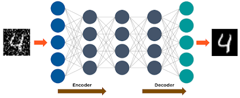
When an image of a digit is not clear, it goes to an autoencoder neural network.
Autoencoders first encode the image, then reduce the size of the input into a smaller representation.
Finally, the autoencoder decodes the image to produce the reconstructed image.
The following image shows how autoencoders work:



Comments
Post a Comment