Meta Pseudo Labels (MPL) Algorithm

 Meta Pseudo Labels (MPL) is a machine learning algorithm that has gained popularity in recent years due to its effectiveness in semi-supervised learning. Semi-supervised learning refers to the task of training a model using both labeled and unlabeled data to improve its accuracy. MPL takes this a step further by using the predictions of a model on unlabeled data to generate "pseudo-labels" and then uses these labels to retrain the model.

Pseudo Meta Labels

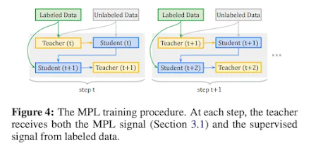
The idea behind MPL is simple: if a model is confident in its predictions on unlabeled data, then those predictions can be used as pseudo-labels to train the model further. The process involves two phases: the first phase trains a model on labeled data, and the second phase uses the trained model to predict labels on unlabeled data, which are then used to retrain the model. The process is repeated until the model converges.

One of the key advantages of MPL is its ability to leverage large amounts of unlabeled data, which is often abundant but expensive to label. By using pseudo-labels, MPL can effectively create "free" labeled data, improving the accuracy of the model without the need for additional human labeling.

Another benefit of MPL is its ability to improve model generalization. When a model is trained on a limited amount of labeled data, it may overfit to the training data and perform poorly on new, unseen data. By incorporating unlabeled data through pseudo-labeling, MPL can help the model learn more generalizable features and reduce overfitting.

Furthermore, MPL has been shown to outperform other semi-supervised learning methods, such as self-training and co-training, in various tasks and datasets. This is due to its ability to learn from both labeled and unlabeled data and generate high-quality pseudo-labels.

Source: https://arxiv.org/abs/2003.10580

When implementing MPL in PyTorch, there are a few additional considerations to keep in mind. One is the choice of loss function. Typically, a combination of supervised and unsupervised loss functions is used to train the model, with the unsupervised loss function based on the consistency between the model's predictions on the labeled and unlabeled data. Another consideration is the choice of optimizer and learning rate, which can have a significant impact on model performance.

Overall, Meta Pseudo Labels is a powerful algorithm that can help improve model performance in semi-supervised learning tasks. Its implementation in PyTorch is relatively straightforward and can be adapted to various datasets and models. With the increasing availability of unlabeled data, MPL offers a practical solution to leverage this data and improve model accuracy and generalization.

Pytorch Implementation of Pseudo Meta Labels

Implementing MPL in PyTorch is straightforward, and there are many resources available online to help guide you through the process. One popular approach involves creating a custom PyTorch Dataset that can handle both labeled and unlabeled data. During training, the model is first trained on labeled data using standard supervised learning techniques. In the second phase, the model is used to generate pseudo-labels for the unlabeled data, and these pseudo-labels are added to the training data. The model is then retrained on the combined dataset, incorporating the newly labeled data.

One important consideration when implementing MPL is the choice of threshold for pseudo-labeling. Setting the threshold too low can result in noisy pseudo-labels, while setting it too high can result in limited use of unlabeled data. Tuning the threshold can be done through experimentation or using techniques such as cross-validation.

Here's an example PyTorch code for the Meta Pseudo Labels algorithm:

import torch
import torch.nn as nn
import torch.optim as optim
from torch.utils.data import DataLoader, Dataset
class CustomDataset(Dataset):
    def __init__(self, labeled_data, unlabeled_data):
        self.labeled_data = labeled_data
        self.unlabeled_data = unlabeled_data
    def __len__(self):
        return len(self.labeled_data) + len(self.unlabeled_data)
    def __getitem__(self, index):
        if index < len(self.labeled_data):
            data, label = self.labeled_data[index]
            return data, label
        else:
            index = index - len(self.labeled_data)
            data = self.unlabeled_data[index]
            return data, -1
class CustomModel(nn.Module):
    def __init__(self):
        super(CustomModel, self).__init__()
        self.conv1 = nn.Conv2d(3, 32, 3, 1, 1)
        self.conv2 = nn.Conv2d(32, 64, 3, 1, 1)
        self.fc1 = nn.Linear(64*8*8, 128)
        self.fc2 = nn.Linear(128, 10)
        self.dropout = nn.Dropout(0.5)
        self.pool = nn.MaxPool2d(2, 2)
        self.relu = nn.ReLU()
    def forward(self, x):
        x = self.conv1(x)
        x = self.relu(x)
        x = self.pool(x)
        x = self.conv2(x)
        x = self.relu(x)
        x = self.pool(x)
        x = x.view(-1, 64*8*8)
        x = self.fc1(x)
        x = self.relu(x)
        x = self.dropout(x)
        x = self.fc2(x)
        return x
def generate_pseudo_labels(model, unlabeled_loader, device, threshold):
    pseudo_labels = []
    model.eval()
    with torch.no_grad():
        for data, _ in unlabeled_loader:
            data = data.to(device)
            output = model(data)
            pred = output.max(1)[1]
            confidence = output.softmax(dim=1).max(1)[0]
            mask = (confidence > threshold).nonzero().squeeze()
            if len(mask) > 0:
                pseudo_labels.append((data[mask], pred[mask]))
    return pseudo_labels
def filter_pseudo_labels(pseudo_labels, model, device, threshold):
    filtered_pseudo_labels = []
    model.eval()
    with torch.no_grad():
        for data, preds in pseudo_labels:
            data = data.to(device)
            output = model(data)
            confidence = output.softmax(dim=1).max(1)[0]
            mask = (confidence > threshold).nonzero().squeeze()
            if len(mask) > 0:
                filtered_preds = preds[mask]
                filtered_pseudo_labels.append((data[mask], filtered_preds))
    return filtered_pseudo_labels
def train_mpl(train_loader, unlabeled_loader, optimizer, criterion, num_epochs, threshold=0.95, alpha=0.75):
    device = torch.device("cuda" if torch.cuda.is_available() else "cpu")
    # Initialize model and EMA model
    model = CustomModel()
    ema_model = CustomModel()
    ema_model.load_state_dict(model.state_dict())
    # Train the model for num_epochs epochs
    for epoch in range(num_epochs):
        train_loss = 0.0
        train_acc = 0.0
        num_unlabeled = 0
        pseudo_labels = []
        # Generate pseudo-labels for unlabeled data
        model.eval()
        with torch.no_grad():
            for data in unlabeled_loader:
                data = data.to(device)
                output = model(data)
                probs = torch.softmax(output, dim=1)
                max_probs, preds = torch.max(probs, dim=1)
                for i, max_prob in enumerate(max_probs):
                    if max_prob > threshold:
                        num_unlabeled += 1
                        pseudo_labels.append((data[i], preds[i]))
        # Filter out unreliable pseudo-labels
        filtered_pseudo_labels = []
        for data, pseudo_label in pseudo_labels:
            with torch.no_grad():
                output = model(data.unsqueeze(0))
                probs = torch.softmax(output, dim=1)
                max_probs, _ = torch.max(probs, dim=1)
                if max_probs.item() > threshold:
                    filtered_pseudo_labels.append((data, pseudo_label))
        # Train the model on labeled data
        model.train()
        for data, label in train_loader:
            data = data.to(device)
            label = label.to(device)
            optimizer.zero_grad()
            output = model(data)
            loss = criterion(output, label)
            loss.backward()
            optimizer.step()
            train_loss += loss.item()
            _, pred = torch.max(output, 1)
            train_acc += (pred == label).sum().item()
        # Train the model on labeled and pseudo-labeled data
        model.train()
        for data, pseudo_label in filtered_pseudo_labels:
            data = data.to(device)
            pseudo_label = pseudo_label.to(device)
            optimizer.zero_grad()
            output = model(data)
            loss = criterion(output, pseudo_label)
            loss.backward()
            optimizer.step()
            train_loss += alpha * loss.item()
            _, pred = torch.max(output, 1)
            train_acc += (pred == pseudo_label).sum().item()
        train_loss /= len(train_loader.dataset) + len(pseudo_labels)
        train_acc /= len(train_loader.dataset) + len(pseudo_labels)
        # Update EMA model
        for param, ema_param in zip(model.parameters(), ema_model.parameters()):
            ema_param.data.mul_(alpha).add_(1 - alpha, param.data)
        # Evaluate the model on the validation set
        ema_model.eval()
        valid_loss = 0.0
        valid_acc = 0.0
        with torch.no_grad():
            for data, label in valid_loader:
                data = data.to(device)
                label = label.to(device)
                output = ema_model(data)
                loss = criterion(output, label)
                valid_loss += loss.item()
                _, pred = torch.max(output, 1)
                valid_acc += (pred == label).sum().item()
        valid_loss /= len(valid_loader.dataset)
        valid_acc /= len(valid_loader.dataset)
  # Print the training and validation metrics for the current epoch
    print(f"Epoch {epoch+1}/{num_epochs} - Train Loss: {train_loss:.4f}, Train Acc: {train_acc:.4f}, Valid Loss: {valid_loss:.4f}, Valid Acc: {valid_acc:.4f}")
return ema_model

In this example code, the `train_mpl` function implements the Meta Pseudo Labels algorithm, including the generation and filtering of pseudo-labels, and the addition of pseudo-labeled data to the training set. The code also includes the implementation of an exponentially moving average of the model parameters, which is used to update the model weights at each epoch.

Conclusion

In conclusion, MPL is a powerful algorithm that can significantly improve the accuracy of models in semi-supervised learning tasks. Its implementation in PyTorch is straightforward and can be easily adapted to different datasets and models. With the abundance of unlabeled data available, MPL offers a practical solution to leverage this data and improve model performance.