How to create a 1D- CNN in TensorFlow

 Several studies concentrate on two-dimensional convolutional neural networks. They are especially useful in image recognition problems. 1D CNNs are covered in some detail, for example, in natural language processing (NLP). Few articles, however, provide an explanatory walkthrough on how to build a 1D-CNN for other machine-learning problems that you may be facing. This article attempts to bridge that chasm.

When to Apply a 1D CNN?

A CNN is effective at identifying simple patterns in data, which are then used to form more complex patterns in higher layers. When you expect to derive interesting features from shorter (fixed-length) segments of the overall data set and the location of the feature within the segment is not important, a 1D CNN is very effective.

This is applicable to the analysis of sensor data time sequences (such as gyroscope or accelerometer data). It also applies to the analysis of any type of signal data over a predetermined time period (such as audio signals). Another application is NLP (although here LSTM networks are more promising since the proximity of words might not always be a good indicator for a trainable. 

Other applications for CNN in sequential data include audio, time series, and natural language processing (NLP). It is widely used for image, audio, video, text, and time series modeling applications. CNN is classified into the following types: 1D Convolution is commonly used when the input data is sequential, such as text or audio. 2D Convolution: This method is used when the input data is an image. 3D Convolution: It is widely used in medical applications such as medical imaging and event detection in videos.

TensorFlow Implementation of 1D-CNN

import tensorflow as tf

from tensorflow.keras.layers import Conv1D, MaxPooling1D, Flatten, Dense, Dropout


# Define the model architecture

model = tf.keras.Sequential([

    Conv1D(filters=64, kernel_size=3, activation='relu', input_shape=(1000, 1)),

    Conv1D(filters=64, kernel_size=3, activation='relu'),

    MaxPooling1D(pool_size=2),

    Conv1D(filters=128, kernel_size=3, activation='relu'),

    Conv1D(filters=128, kernel_size=3, activation='relu'),

    MaxPooling1D(pool_size=2),

    Conv1D(filters=256, kernel_size=3, activation='relu'),

    Conv1D(filters=256, kernel_size=3, activation='relu'),

    MaxPooling1D(pool_size=2),

    Flatten(),

    Dense(512, activation='relu'),

    Dropout(0.5),

    Dense(256, activation='relu'),

    Dropout(0.5),

    Dense(1, activation='sigmoid')

])

# Compile the model

model.compile(optimizer='adam', loss='binary_crossentropy', metrics=['accuracy'])

# Train the model

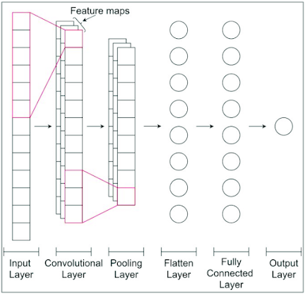
model.fit(x_train, y_train, validation_data=(x_test, y_test), epochs=50, batch_size=32)

In this example, the model architecture consists of multiple convolutional layers with varying filter sizes and max pooling layers to extract relevant features from the ECG data. The Flatten layer is used to convert the output of the convolutional layers to a 1D tensor that can be passed through fully connected layers. The Dropout layers are used to prevent overfitting. Finally, the sigmoid activation function is used in the output layer to output a probability of the input belonging to a certain class. The model is trained using the binary crossentropy loss function and the Adam optimizer.