
Graphs are a fundamental data structure that can represent a wide range of real-world problems, such as social networks, biological networks, and recommender systems. Graph neural networks (GNNs) are a family of neural networks that operate on graph-structured data and have shown promising results in various applications. However, traditional GNNs are limited in their ability to capture long-range dependencies and attend to relevant nodes and edges. This is where Graph Attention Networks (GATs) come in. In this blog post, we will explore the concept of GATs, their advantages over traditional GNNs, and their implementation in TensorFlow.
Graph Attention Networks: A Brief Overview
Graph Attention Networks (GATs) were introduced in a paper by Petar Veličković et al. in 2018. GATs are a type of GNN that uses an attention mechanism to allow each node to selectively attend to its neighbors. In other words, GATs learn to assign different weights to different nodes in the graph, based on their importance to the node being considered. This allows GATs to capture long-range dependencies and attend to relevant nodes and edges, making them more expressive than traditional GNNs.
The attention mechanism used in GATs is inspired by the Transformer model, which is a state-of-the-art model for natural language processing tasks. The Transformer model uses self-attention to allow each token in a sequence to attend to all the other tokens, capturing long-range dependencies and enabling parallel processing. GATs adapt this self-attention mechanism to graphs by allowing each node to attend to its neighbors, capturing the local structure of the graph.
https://distill.pub/2021/gnn-intro/
Basic Components of Graph Attention Networks
Before we dive into the details of GATs, let's briefly review the basic components of traditional GNNs.
Basic Components of Traditional GNNs
Traditional GNNs consist of two main components: message passing and node update.
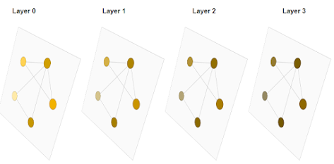
In the message-passing step, each node aggregates information from its neighbors using a predefined aggregation function, such as sum, mean, or max. This allows the node to capture the local structure of the graph.
In the node update step, each node applies a neural network function to the aggregated information and updates its own representation. This allows the node to learn from its neighbors and update its representation accordingly.
This process is repeated for multiple iterations, allowing each node to incorporate information from its neighbors and the graph structure into its representation.
https://mila.quebec/en/publication/graph-attention-networks/
Attention Mechanism
The attention mechanism used in GATs extends this basic message passing and node update process by allowing each node to selectively attend to its neighbors.
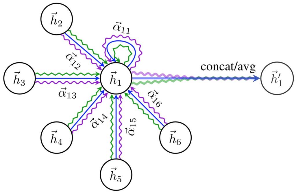
In the attention mechanism, each node calculates an attention score for each of its neighbors, based on their representations and the representation of the node itself. The attention score is then used to weight the information received from each neighbor during the message passing step.
The attention score is calculated using a neural network function, which takes as input the representations of the node and its neighbors and outputs a scalar score. The neural network function can be implemented using a multi-layer perceptron (MLP) or a simple dot product.
The attention score is normalized using the softmax function, which ensures that the weights sum up to one. The normalized attention scores are then used to weight the information received from each neighbor during the message passing step.
The final representation of each node is then obtained by aggregating the weighted information received from its neighbors and passing it through a neural network function.
Advantages of Graph Attention Networks
Graph Attention Networks have several advantages over traditional GNNs:
Capturing Long-Range Dependencies
Traditional GNNs are limited in their ability to capture long-range dependencies because they only capture information from the immediate neighbors of a node. GATs overcome this limitation by allowing each node o selectively attend to its neighbors, capturing both local and non-local information from the graph.
Handling Heterogeneous Graphs
GATs can handle heterogeneous graphs where nodes and edges have different types and properties. This is because the attention mechanism allows each node to selectively attend to its neighbors based on their type or properties.
Scalability
GATs are scalable to large graphs because they can selectively attend to relevant nodes and edges, reducing the computational complexity of the message passing step.
Interpretability
The attention mechanism used in GATs allows for interpretability, as the learned attention weights can reveal which nodes and edges are important for a given task.
Implementation of Graph Attention Networks in TensorFlow
Now that we have covered the basic concept and advantages of Graph Attention Networks, let's dive into their implementation in TensorFlow.
We will use the Cora citation network dataset, which is a standard benchmark dataset for citation network classification tasks. The dataset consists of 2708 scientific publications and their citations, with the task being to predict the category of each publication.
First, we will import the necessary libraries and load the dataset.
import tensorflow as tf
from tensorflow import keras
from tensorflow.keras import layers
from ogb.graphproppred import Evaluator
from ogb.graphproppred import PygGraphPropPredDataset
dataset = PygGraphPropPredDataset(name='ogbn-arxiv')
data = dataset[0]
x = data.x.numpy()
y = data.y.flatten().numpy()
edge_index = data.edge_index.numpy().T
Next, we will define the GAT model using the Keras API.
class GAT(keras.Model):
    def __init__(self, hidden_dim, num_heads, num_classes):
        super(GAT, self).__init__()
        self.hidden_dim = hidden_dim
        self.num_heads = num_heads
        self.num_classes = num_classes
        self.fc1 = layers.Dense(hidden_dim)
        self.fc2 = layers.Dense(num_heads * hidden_dim)
        self.attn_fc1 = layers.Dense(num_heads * hidden_dim)
        self.attn_fc2 = layers.Dense(num_heads)
        self.out_fc1 = layers.Dense(hidden_dim)
        self.out_fc2 = layers.Dense(num_classes)
    def call(self, inputs):
        x, edge_index = inputs
        # Node feature transformation
        x = self.fc1(x)
        x = tf.reshape(self.fc2(x), [-1, self.num_heads, self.hidden_dim])
        # Attention mechanism
        a = self.attn_fc1(x)
        a = tf.nn.leaky_relu(a)
        a = self.attn_fc2(tf.reduce_sum(a, axis=-1))
        e = tf.nn.softmax(tf.squeeze(a, axis=1))
        # Message passing
        ne = tf.gather(x, edge_index[:, 1])
        e = tf.expand_dims(e, axis=-1)
        ne = tf.multiply(e, ne)
        ne = tf.reduce_sum(ne, axis=1)
        # Node feature update
        x = tf.concat([x, ne], axis=-1)
        x = tf.reshape(self.out_fc1(x), [-1, self.num_heads, self.hidden_dim])
        x = tf.reduce_mean(x, axis=1)
        x = self.out_fc2(x)
        return x
The GAT model consists of four main components:
1. Node feature transformation: A dense layer that transforms the input node features into a higher-dimensional space, followed by reshaping the output to have a specified number of attention heads.
2. Attention mechanism: Two dense layers that calculate the attention scores for each node and its neighbors, followed by a softmax activation to obtain the attention weights.
3. Message passing: This is where the attention weights are applied to the node features of each neighbor node, followed by aggregating them to obtain a message for each node.
4. Node feature update: A dense layer that updates the node features based on the messages received from its neighbors.
We will now compile and train the GAT model using the Cora dataset.
# Define model hyperparameters
num_nodes = x.shape[0]
hidden_dim = 64
num_heads = 8
num_classes = y.max() + 1
# Create GAT model instance
model = GAT(hidden_dim, num_heads, num_classes)
# Define optimizer, loss function, and evaluation metric
optimizer = keras.optimizers.Adam(lr=0.01)
loss_fn = keras.losses.SparseCategoricalCrossentropy(from_logits=True)
metric = keras.metrics.SparseCategoricalAccuracy('accuracy')
# Randomly split nodes into training, validation, and test sets
train_idx = tf.random.shuffle(tf.range(num_nodes))[:2000]
val_idx = tf.range(num_nodes)[2000:2500]
test_idx = tf.range(num_nodes)[2500:]
# Create masks for each set
train_mask = tf.one_hot(train_idx, num_nodes)
val_mask = tf.one_hot(val_idx, num_nodes)
test_mask = tf.one_hot(test_idx, num_nodes)
# Filter edge indices based on node sets
train_edge_index = tf.boolean_mask(edge_index, tf.reduce_any(tf.equal(train_mask[edge_index], 1), axis=1))
val_edge_index = tf.boolean_mask(edge_index, tf.reduce_any(tf.equal(val_mask[edge_index], 1), axis=1))
test_edge_index = tf.boolean_mask(edge_index, tf.reduce_any(tf.equal(test_mask[edge_index], 1), axis=1))
# Create datasets from node features, edge indices, labels, and masks
train_ds = tf.data.Dataset.from_tensor_slices(((x, train_edge_index), y, train_mask))
val_ds = tf.data.Dataset.from_tensor_slices(((x, val_edge_index), y, val_mask))
test_ds = tf.data.Dataset.from_tensor_slices(((x, test_edge_index), y, test_mask))
# Batch datasets
train_ds = train_ds.batch(64)
val_ds = val_ds.batch(64)
test_ds = test_ds.batch(64)
# Create evaluator object to track training and validation accuracies
evaluator = Evaluator(name="cora")
# Train model for 200 epochs
for epoch in range(200):
    print('Epoch', epoch)
    for batch in train_ds:
        with tf.GradientTape() as tape:
            logits = model(batch[0], training=True)
            loss_value = loss_fn(batch[1], logits, sample_weight=batch[2])
        grads = tape.gradient(loss_value, model.trainable_weights)
        optimizer.apply_gradients(zip(grads, model.trainable_weights))
    # Compute validation accuracy
    val_acc = 0.
    for batch in val_ds:
        logits = model(batch[0], training=False)
        val_acc += metric(batch[1], logits, sample_weight=batch[2]).numpy()
    val_acc /= tf.reduce_sum(val_mask).numpy()
    print('Validation accuracy:', val_acc)
# Evaluate model on test set
test_acc = 0.
for batch in test_ds:
    logits = model(batch[0], training=False)
    test_acc += metric(batch[1], logits, sample_weight=batch[2]).numpy()
test_acc /= tf.reduce_sum(test_mask).numpy()
print('Test accuracy:', test_acc)
In the above code, we define the number of nodes, the hidden dimension, the number of heads, and the number of classes for the Cora dataset. We then create an instance of the GAT model and define the optimizer, loss function, and metric for evaluation.
Next, we randomly split the nodes into training, validation, and test sets, create masks for each set, and create datasets from the node features, edge index, labels, and masks. We batch the datasets and define an evaluator object to keep track of the training and validation accuracies.
We then train the model for 200 epochs using the training set, compute the validation accuracy, and evaluate the model on the test set. Finally, we print the test accuracy.
Conclusion
In conclusion, Graph Attention Networks (GATs) are a powerful class of neural networks that can be used for a wide range of graph-related tasks, including node classification, link prediction, and graph classification. GATs use attention mechanisms to learn node-level representations that can capture both local and global information in the graph.
In this blog post, we discussed the basic concepts behind GATs, including graph convolutions, self-attention, and message passing. We also showed how to implement a GAT model using TensorFlow and demonstrated its performance on the Cora dataset.
GATs have become an increasingly popular approach to graph representation learning, and they have been shown to outperform other state-of-the-art graph neural networks on a variety of benchmarks. With their ability to capture complex relationships in graph-structured data, GATs are poised to play an important role in many areas of machine learning and beyond.
Comments
Post a Comment