
In this post, we will review and summarize the Swin Transformer paper, titled as Swin Transformer: Hierarchical Vision Transformer using Shifted Windows. Some of the code used here will be obtained from this Github Repo, so you better clone it in case you want to test some of this work, However, the aim of this post is to better simplify and summarize the Swin transformer paper. Soon, there will be another Post explaining how to implement the Swin Transformer in details.
Overview
The "Swin Transformer: Hierarchical Vision Transformer using Shifted Windows" is a research paper that proposes a new architecture for visual recognition tasks using a hierarchical transformer model. The architecture, called the Swin Transformer, uses a combination of local and global attention mechanisms to process images and improve the accuracy of image classification and object detection tasks. The Swin Transformer uses a series of shifted window attention mechanisms to enable the model to focus on different parts of the image at different scales, and a hierarchical structure to allow the model to learn and reason about the relationships between different image regions. The authors of the paper claim that the Swin Transformer outperforms existing transformer-based models on a number of benchmark datasets and tasks.
To be clear and at the same time not oversimplify this work, there are a few key concepts that Swin Transformer proposed and they are built on top of ViT to get their complete grasp of the new model's architecture. The two concepts are:
- Shifted Window Attention
- Patch Merging
The rest of the Swin Transformer's architecture seems pretty much as the same as ViT (with some small modifications). Hence, what are the two concepts? We will explain them later in this blog post.
First, let’s get a deeper overview of the architecture.
What makes it different than ViT?
The Swin Transformer is an extension of the Vision Transformer (ViT) model, which was introduced in the paper "An Image is Worth 16x16 Words: Transformers for Image Recognition at Scale" (https://arxiv.org/abs/2010.11929). Like ViT, the Swin Transformer is a Transformer-based architecture that processes images as a sequence of patches, rather than using convolutional layers as in traditional image recognition models. However, the Swin Transformer introduces several key changes to the ViT architecture to improve performance on visual recognition tasks.
One of the main differences between the Swin Transformer and ViT is the use of shifted window attention mechanisms. In the Swin Transformer, the attention mechanisms operate over a series of shifted windows of different sizes, rather than over the full image as in ViT. This allows the model to attend to different parts of the image at different scales and better capture local relationships between image patches.
The Swin Transformer also introduces a hierarchical structure, where the output of the shifted window attention mechanisms at each scale is passed through a separate transformer layer before being combined and passed to the next scale. This hierarchical structure allows the model to learn and reason about the relationships between different image regions at different scales.
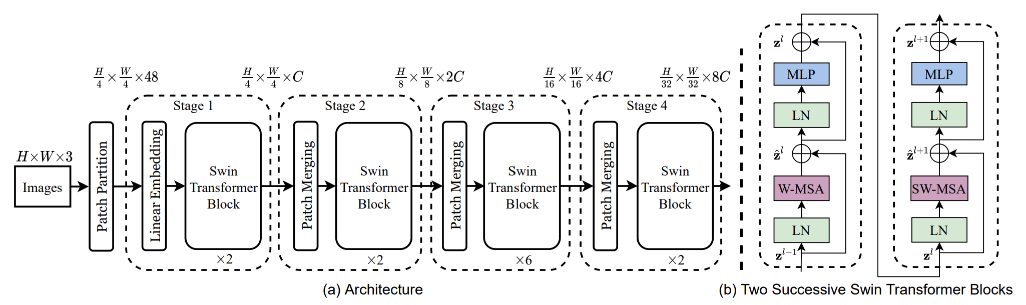
The Swin Transformer architecture is shown in the figure above, with the tiny version (SwinT) depicted. Like the Vision Transformer (ViT), it begins by dividing an input RGB image into non-overlapping patches using a patch-splitting module. Each patch is treated as a "token" and its features are the concatenated RGB values of the raw pixels. In this implementation, the patches are 4x4 in size and therefore have a feature dimension of 4x4x3=48. A linear embedding layer is then applied to this raw-valued feature to project it to a different dimension (denoted as C).
Patch Partition (From section 3.1 of the paper):
The first step in the process is to input an image and convert it to patch embeddings, which is the same as in ViT. The difference is that the patch size in the Swin Transformer is 4x4 instead of 16x16 as in ViT. Patch embeddings have previously been explained here.
from timm.models.layers import PatchEmbed
x = torch.randn(1, 3, 224, 224)
patch_embed = PatchEmbed(img_size=224, patch_size=4, embed_dim=96)
patch_embed(x).shape
 torch.Size([1, 3136, 96])
As can be seen, the output of the Patch Embedding layer is of shape (1,3136,96), that is (1, H/4, W/4, 96), where 96 is the embedding dimension C.
stage_1 = BasicLayer(dim=96, out_dim=192,
                     input_resolution=(56, 56),
                     depth=2)
inp = torch.randn(1, 56*56, 96)
stage_1(inp).shape
 torch.Size([1, 3136, 96])
As shown in the code snippet, the dimensions of the input do not change as it passes through "Stage 1". In fact, the dimensions remain constant as the input passes through every stage. It is only between stages that a patch merging layer is applied to reduce the number of tokens as the network becomes deeper.
Path Merging Layer
The first patch merging layer combines the features of groups of 2x2 neighboring patches and applies a linear layer on the concatenated features, which have a dimension of 4C. This reduces the number of tokens by a factor of 4 (corresponding to a 2x downsampling of resolution), and the output dimension is set to 2C. In this case, C is the number of channels (embedding dimension) and is equal to 96 for the tiny version of the Swin Transformer described in this blog post.
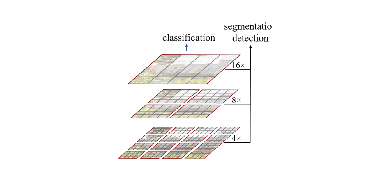
The patch-merging layer merges four patches at a time, so with each merge the height and width of the image are reduced by a factor of 2. For example, in stage 1 the input resolution is (H/4, W/4), but after patch merging the resolution becomes (H/8, W/8), which is the input for stage 2. Similarly, the input resolution for stage 3 is (H/16, W/16) and for stage 4 it is (H/32, W/32). The patch-merging process can be understood by examining the inputs and outputs in the code.
from timm.models.swin_transformer import PatchMerging
x = torch.randn(1, 56*56, 96)
l = PatchMerging(input_resolution=(56, 56), dim=96, out_dim=192, norm_layer=nn.LayerNorm)
l(x).shape
torch.Size([1, 784, 192]) # (1, 28x28, 192)
As shown, the output width and height are both reduced by a factor of 2, and the number of output channels is 2C where C is the number of input channels. In the case of the Swin-T model, C=96. The source code for patch merging can be examined to further understand its function.
class PatchMerging(nn.Module):
    def __init__(self, input_resolution, dim, out_dim=None, norm_layer=nn.LayerNorm):
        super().__init__()
        self.input_resolution = input_resolution
        self.dim = dim
        self.out_dim = out_dim or 2 * dim
        self.norm = norm_layer(4 * dim)
        self.reduction = nn.Linear(4 * dim, self.out_dim, bias=False)
    def forward(self, x):
        """
        x: B, H*W, C
        B: Batch size
        """
        H, W = self.input_resolution
        B, L, C = x.shape
        x = x.view(B, H, W, C)
        x0 = x[:, 0::2, 0::2, :]  # B H/2 W/2 C
        x1 = x[:, 1::2, 0::2, :]  # B H/2 W/2 C
        x2 = x[:, 0::2, 1::2, :]  # B H/2 W/2 C
        x3 = x[:, 1::2, 1::2, :]  # B H/2 W/2 C
        x = torch.cat([x0, x1, x2, x3], -1)  # B H/2 W/2 4*C
        x = x.view(B, -1, 4 * C)  # B H/2*W/2 4*C
        x = self.norm(x)
        x = self.reduction(x)
        return x
Deeper Dive into Shifted Windows Mechanism (From section 3.2 of the paper):
In the Swin Transformer, the attention mechanisms operate over a series of shifted windows of different sizes, rather than over the full image as in the original Vision Transformer (ViT) model. Each window consists of a set of image patches, and the model uses attention to weight the importance of each patch within the window. The size of the window and the number of patches it contains can vary, and the model can use different window sizes for different scales of image information.
The use of shifted windows allows the model to attend to different parts of the image at different scales, rather than just processing the entire image at a single scale as in ViT. This enables the model to better capture local relationships between image patches, as it can focus on a small region of the image and attend to the patches within that region.
The attention mechanisms in the Swin Transformer are similar to those used in other transformer models. They use a dot product between the query and key vectors to compute the attention weights for each patch within the window. The model then uses these attention weights to compute a weighted sum of the value vectors for each patch, which is used as input to the next layer of the model.
As shown in the figure, the first module uses a regular window partitioning strategy that begins at the top-left pixel and evenly divides the 8x8 feature map into 2x2 windows of size 4x4 (M=4). The next module uses a windowing configuration that is shifted from the previous layer by [M/2] pixels in both the x and y dimensions ([M/2], [M/2]). This is illustrated in the figure below:
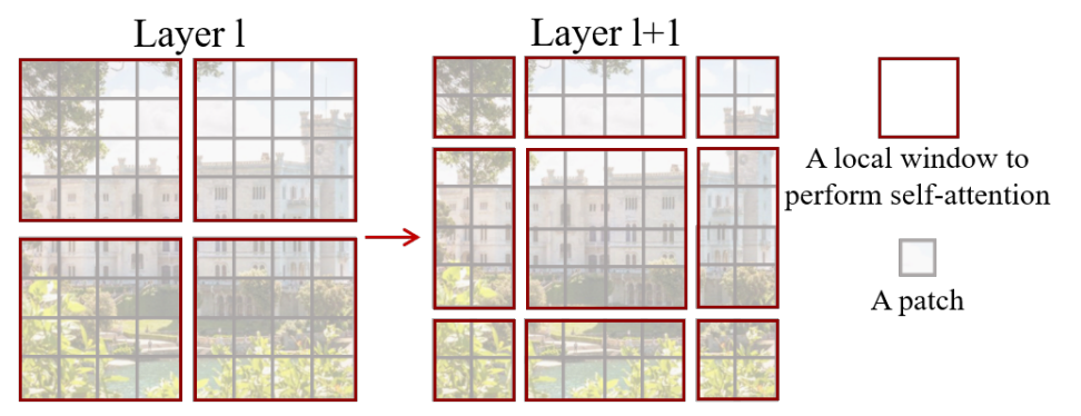
As seen, the left image shows an 8x8 feature map that is evenly divided into 4 windows of size 4x4. The window size is M=4. In the first part of the two successive blocks, attention is calculated within these windows. However, the network also needs cross-window attention to learn better, because it is no longer using a global context. To achieve this, the second part of the Swin Transformer block shifts the windows by ([M/2], [M/2]) pixels from their regular positions and performs attention between the new windows, leading to cross-window connections. In this case, since M=4, the windows are displaced by (2,2). Self-attention is then performed inside the shifted local windows.
To implement the shifted window mechanism in PyTorch, you can use the torch.nn.UniformPatch2d function to extract patches from the input tensor and apply a sliding window operation with a specified stride. Here is an example of how this could be done:
import torch
# Input tensor with size (batch_size, channels, height, width)
x = torch.randn(batch_size, channels, height, width)
# Set the patch size and stride
patch_size = 4
stride = 2
# Create a UniformPatch2d object with the specified patch size and stride
patch_sampler = torch.nn.UniformPatch2d(patch_size, stride)
# Extract patches from the input tensor using the patch sampler
patches = patch_sampler(x)
# Patches has size (batch_size, channels, num_patches_height, num_patches_width, patch_size, patch_size)
Swin Transformer Experiments
It seems that the Swin Transformer models outperform other vision transformer models (such as DeiT and ViT) and are comparable with EfficientNet and RegNet models when trained from scratch on the ImageNet-1K dataset. Additionally, the Swin Transformer models may have a slightly better speed-accuracy trade-off compared to EfficientNet and RegNet models. This suggests that the Swin Transformer architecture is effective for visual recognition tasks and may be a promising alternative to other state-of-the-art models.
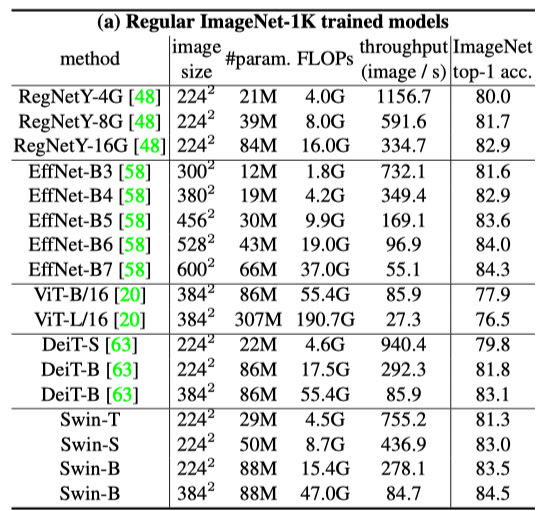
It appears that the Swin Transformer model is a modification of the standard transformer architecture and has some potential for further improvement. This is in contrast to EfficientNet and RegNet models, which are the result of extensive architecture searches. This suggests that the Swin Transformer architecture may be able to achieve even better performance with further optimization or modifications.
At last, the shifted window attention mechanism in the Swin Transformer allows the model to attend to different parts of the image at different scales and better capture local relationships between image patches, which can improve the accuracy of visual recognition tasks.
Comments
Post a Comment