U-Net Implementation For the Segmentation of Nuclei

 

Introduction

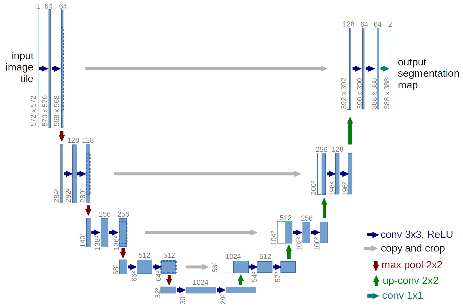
Image segmentation is the partitioning of images into various regions, in which every region has a different entity. An efficient tool for image segmentation is a convolutional neural network (CNN). Recently, there has been a significant impact of CNNs that are designed to perform image segmentation. One the best models presented was the U-Net. A U-Net is U-shaped convolutional neural network that was originally designed to segment biomedical images. Such a network is better than conventional models, in terms of architecture and pixel-based image segmentation formed from convolutional neural network layers. Similar to all CNNs, this network consists of convolution, Max-pooling, and ReLU activation layers. However, in a general view, U-Net can be seen as an encoder-decoder network. The encoder is the first part of this network and it is a conventional convolutional neural network like VGG or ResNet that is composed of convolution, pooling, and downsampling layers used to learn some feature maps of the input images. The decoder part is the upsampling and concatenation part which is meant to semantically project the learned discriminative features (lower resolution) by the encoder part onto the pixel space (higher resolution) to get a dense classification.

 

 What is interesting and quite new in the decoder part is the upsampling, which is not usually used in the case of classification or object detection. The idea of it is that the network needs to restore the features maps learn by the encoder to their original size of the input image. Hence, to do so we need to expand the dimensions of the features using transposed convolutions or upconvolution; also called upsampling.

U-Net has shown great efficiency and accuracy when applied to various segmentation tasks in medicine and other fields. Moreover, such a network has also shown good performance when training datasets is quite small. Thus, in this article, we will implement a U-Net using Keras Library. The network will be built and trained using a medical dataset named nuclei. After training, the network must be capable of segmenting a nucleus in a cell image.

U-Net Implementation for Nuclei Segmentation

In this work, we will implement a U-Net for segmenting or detecting the nuclei in images. The U-Net implementation will undergo 4 stages:

•    Loading Dataset
•     Building encoder and decoder
•     Training the U-Net
•     Testing the U-Net

Loading Dataset

A human’s body consists of 40 trillion cells that have a nucleus that is full of DNA. Hence, the detection or identifying nuclei of a cell can be the starting point of most tests and analyses. Moreover, researchers need also to identify the nuclei of cells in order to investigate the reaction of cells to treatments and understand the underlying biological processes at work. Thus, it is important to have an automated and intelligent system for the segmentation of nuclei. Such a system can be best using U-Net.

The dataset that will be used to train and test the build U-Net is the nuclei, found on Kaggle. The dataset consists of many stages however in this work, we will use the train stage 1 and test stage 1, for training and testing, respectively. Once, you download the dataset you find out that training images consist of a file called images, which have images of cells in addition to their associated ImageIDs. The training images file has also a separate file for every image’s mask. Hence, our code here should read original images in addition to their masks by their ImageIDs. 

Before loading the dataset, let’s first load some libraries and packages we will need when building the network.

import tensorflow as tf

import os

import sys

import numpy as np

from tqdm import tqdm

from itertools import chain

from skimage.io import imread, imshow

from skimage.transform import resize

from tensorflow.compat.v1 import ConfigProto

from tensorflow.compat.v1 import InteractiveSession

config = ConfigProto()

config.gpu_options.allow_growth = True

session = InteractiveSession(config=config)

with that set, let’s load our train images and their corresponding masks.

# tf.enable_eager_execution()

IMG_WIDTH = 128

IMG_HEIGHT = 128

IMG_CHANNELS = 3

DATA_PATH = r'C:/Users/abdul/Downloads/stage1_train/'

seed = 42

np.random.seed = seed

image_ids = next(os.walk(DATA_PATH))[1]

X = np.zeros((len(image_ids), IMG_HEIGHT, IMG_WIDTH, IMG_CHANNELS), dtype=np.uint8)

Y = np.zeros((len(image_ids), IMG_HEIGHT, IMG_WIDTH, 1), dtype=np.bool)

for n, id_ in tqdm(enumerate(image_ids), total=len(image_ids)):

    path = DATA_PATH + id_

    img = imread(path + '/images/' + id_ + '.png')[:,:,:IMG_CHANNELS]

    img = resize(img, (IMG_HEIGHT, IMG_WIDTH), mode='constant', preserve_range=True)

    X[n] = img

    mask = np.zeros((IMG_HEIGHT, IMG_WIDTH, 1), dtype=np.bool)

    for mask_file in next(os.walk(path + '/masks/'))[2]:

        mask_ = imread(path + '/masks/' + mask_file)

        mask_ = np.expand_dims(resize(mask_, (IMG_HEIGHT, IMG_WIDTH), mode='constant',

                                      preserve_range=True), axis=-1)

        mask = np.maximum(mask, mask_)

    Y[n] = mask

x_train=X

y_train=Y

Building the U-Net

The first part of building the U-Net is building the first part which as discussed above an encoder network that consists of convolution, pooling, and downsampling. We will create a simple convolutional neural network of 5 convolutional layers.

# Build U-Net model

inputs = tf.keras.layers.Input((IMG_HEIGHT, IMG_WIDTH, IMG_CHANNELS))

s = tf.keras.layers.Lambda(lambda x: x / 255)(inputs)

c1 = tf.keras.layers.Conv2D(16, (3, 3), activation=tf.keras.activations.elu, kernel_initializer='he_normal',

                            padding='same')(s)

c1 = tf.keras.layers.Dropout(0.1)(c1)

c1 = tf.keras.layers.Conv2D(16, (3, 3), activation=tf.keras.activations.elu, kernel_initializer='he_normal',

                            padding='same')(c1)

p1 = tf.keras.layers.MaxPooling2D((2, 2))(c1)

c2 = tf.keras.layers.Conv2D(32, (3, 3), activation=tf.keras.activations.elu, kernel_initializer='he_normal',

                            padding='same')(p1)

c2 = tf.keras.layers.Dropout(0.1)(c2)

c2 = tf.keras.layers.Conv2D(32, (3, 3), activation=tf.keras.activations.elu, kernel_initializer='he_normal',

                            padding='same')(c2)

p2 = tf.keras.layers.MaxPooling2D((2, 2))(c2)

c3 = tf.keras.layers.Conv2D(64, (3, 3), activation=tf.keras.activations.elu, kernel_initializer='he_normal',

                            padding='same')(p2)

c3 = tf.keras.layers.Dropout(0.2)(c3)

c3 = tf.keras.layers.Conv2D(64, (3, 3), activation=tf.keras.activations.elu, kernel_initializer='he_normal',

                            padding='same')(c3)

p3 = tf.keras.layers.MaxPooling2D((2, 2))(c3)

c4 = tf.keras.layers.Conv2D(128, (3, 3), activation=tf.keras.activations.elu, kernel_initializer='he_normal',

                            padding='same')(p3)

c4 = tf.keras.layers.Dropout(0.2)(c4)

c4 = tf.keras.layers.Conv2D(128, (3, 3), activation=tf.keras.activations.elu, kernel_initializer='he_normal',

                            padding='same')(c4)

p4 = tf.keras.layers.MaxPooling2D(pool_size=(2, 2))(c4)

c5 = tf.keras.layers.Conv2D(256, (3, 3), activation=tf.keras.activations.elu, kernel_initializer='he_normal',

                            padding='same')(p4)

c5 = tf.keras.layers.Dropout(0.3)(c5)

c5 = tf.keras.layers.Conv2D(256, (3, 3), activation=tf.keras.activations.elu, kernel_initializer='he_normal',

                            padding='same')(c5)

Now, we should hook up this part to the second part of the U-net which is the upsampling or decoder part.

u6 = tf.keras.layers.Conv2DTranspose(128, (2, 2), strides=(2, 2), padding='same')(c5)

u6 = tf.keras.layers.concatenate([u6, c4])

c6 = tf.keras.layers.Conv2D(128, (3, 3), activation=tf.keras.activations.elu, kernel_initializer='he_normal',

                            padding='same')(u6)

c6 = tf.keras.layers.Dropout(0.2)(c6)

c6 = tf.keras.layers.Conv2D(128, (3, 3), activation=tf.keras.activations.elu, kernel_initializer='he_normal',

                            padding='same')(c6)

u7 = tf.keras.layers.Conv2DTranspose(64, (2, 2), strides=(2, 2), padding='same')(c6)

u7 = tf.keras.layers.concatenate([u7, c3])

c7 = tf.keras.layers.Conv2D(64, (3, 3), activation=tf.keras.activations.elu, kernel_initializer='he_normal',

                            padding='same')(u7)

c7 = tf.keras.layers.Dropout(0.2)(c7)

c7 = tf.keras.layers.Conv2D(64, (3, 3), activation=tf.keras.activations.elu, kernel_initializer='he_normal',

                            padding='same')(c7)

u8 = tf.keras.layers.Conv2DTranspose(32, (2, 2), strides=(2, 2), padding='same')(c7)

u8 = tf.keras.layers.concatenate([u8, c2])

c8 = tf.keras.layers.Conv2D(32, (3, 3), activation=tf.keras.activations.elu, kernel_initializer='he_normal',

                            padding='same')(u8)

c8 = tf.keras.layers.Dropout(0.1)(c8)

c8 = tf.keras.layers.Conv2D(32, (3, 3), activation=tf.keras.activations.elu, kernel_initializer='he_normal',

                            padding='same')(c8)

u9 = tf.keras.layers.Conv2DTranspose(16, (2, 2), strides=(2, 2), padding='same')(c8)

u9 = tf.keras.layers.concatenate([u9, c1], axis=3)

c9 = tf.keras.layers.Conv2D(16, (3, 3), activation=tf.keras.activations.elu, kernel_initializer='he_normal',

                            padding='same')(u9)

c9 = tf.keras.layers.Dropout(0.1)(c9)

c9 = tf.keras.layers.Conv2D(16, (3, 3), activation=tf.keras.activations.elu, kernel_initializer='he_normal',

                            padding='same')(c9)

outputs = tf.keras.layers.Conv2D(1, (1, 1), activation='sigmoid')(c9)

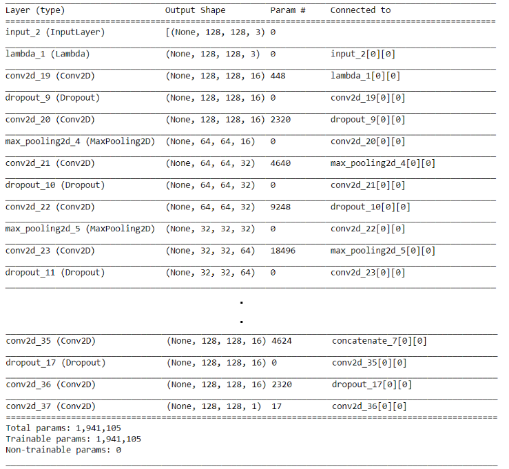
After the network is built, we will define the model and set its optimizer preparing it for the training stage. We will use ADAM as an optimizer and binary cross entropy as a loss function. This will finally get you the final architecture of the designed model. 

model = tf.keras.Model(inputs=[inputs], outputs=[outputs])

model.compile(optimizer='adam', loss='binary_crossentropy', metrics=['accuracy'])

model.summary()

 Training the U-Net

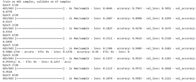
In here, we will feed the loaded images in the first part, to the designed U-Net and train it using all training images keeping 10% for validation. We will set the number of epochs to 20 which must be enough for the network to converge. If not, you can increase the number of epochs.

Network Testing and Evaluation

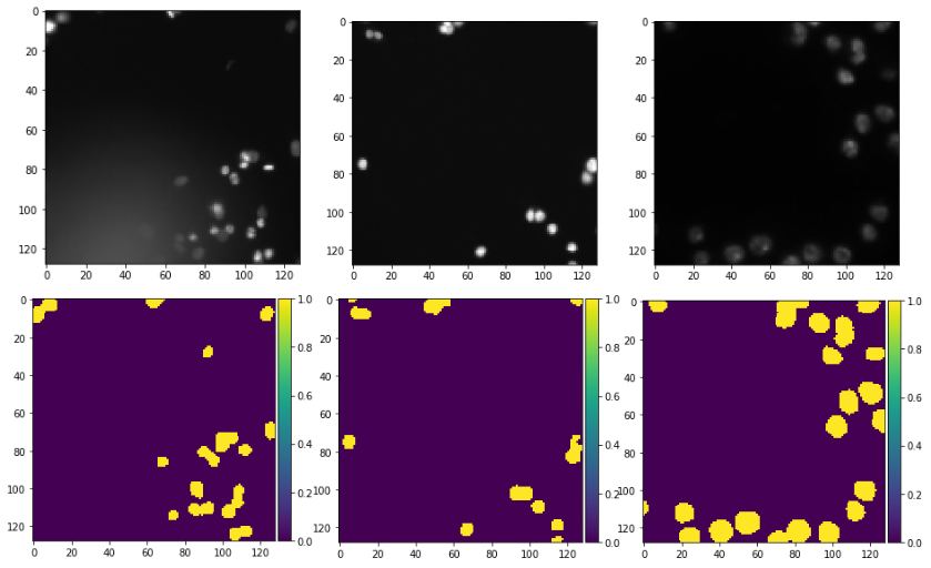
It was seen that network reached a very high accuracy rate at epoch 20, however, the network hasn’t been tested yet on images that were not part of the training set. In this section, we will let the U-Net predict the segmentation output of some testing images and visualize the results.

import matplotlib.pyplot as plt

idx = np.random.randint(0, len(x_test))

x=np.array(x_test[idx])

x=np.expand_dims(x, axis=0)

predict = model.predict(x, verbose=1)

predict = (predict > 0.5).astype(np.uint8)

imshow(np.squeeze(predict[0]))

plt.show()

imshow(x_test[idx])

plt.show()

this will get us images and their segmented outputs as follows:

 

Conclusion

In this article, we implemented a simple U-Net using Keras. The designed U-Net encoder part is a simple deep network, however other pre-trained models can be used such as ResNet and VGGs. Such models can improve the performance of a U-Net as it owns more powerful feature extraction capabilities.